Professional tennis players have unstable working conditions. It’s normal to finish a tournament Sunday in North America and then fly to Europe by Tuesday for another. Even within a continent players often to flit between cities, only staying in one location as long as they’re winning. In 2019, the month of September for many WTA professionals had stops in Zhengzhou, Osaka, Wuhan, and Beijing. I’ve heard players describe their time on tour as a blur of hotel rooms occassionally interrupted by tennis.
Unfortunately, Tennis, the game, contributes to this instability. Although its rules and dimensions don’t change, almost everything else about it does. It is the only major sport that literally changes under your feet. Depending on the season, a tennis match can be played on an acrylic surface, loosely-packed clay, or prim british grass. Each category has its own divisions. So-called “hard courts” might be permanent installations — like the courts at your neighborhood park — built on poured concrete. Or, they could be temporary courts laid down in a stadium for a tournament. Clay courts can be made out of thin green American “har-tru,” thick red European dirt, or, for a moment in time, blue Spanish clay. Grass courts inherit their taxonomy from botany. Wimbledon uses 100% Perennial Ryegrass trimmed to 8mm. Other venues use creeping Bermuda grass or Bentgrass which interact with the tennis ball in slightly different ways.
The tennis ball itself also varies from venue to venue. Different brands of ball use slightly different materials, leading to different performance. Some balls play fast and others are liable to “fluff up” and play slow. The same tournament, hosting both men’s and women’s events, may use slightly different balls for both genders. Pros playing mixed doubles will note how the ball in their current match differs from the one used in singles, allowing them to hit their shots a little faster or slower.
Quantifying play conditions
These differences between courts and balls are important. Both contribute to the “speed” of play conditions. Fast conditions — like a grass court played with light balls — benefit players with a certain style. Slow conditions — think clay — benefit a different style. The degree conditions help, or hinder, a player can be significant. If someone asks you who would win between Jannik Sinner and Carlos Alcaraz, your first question should be “under what conditions?” If it’s clay, bet on Alcaraz. If it’s grass, Sinner likely has the edge.
For how important court and ball type are, their effects on condition speed are hard to quantify. A “court pace index” exists that is calcuated with the Hawk-Eye ball tracking system, though it’s rarely published. Short of actually playing in the tournament and experiencing how fast the ball goes, the best people like us can do is eyeball speeds by watching matches.
Jeff Sackman, though, has a clever workaround. We don’t have Hawk-Eye data, but we do have ace data, and aces contain ample information about the speed of play conditions. Generally, more aces means quicker conditions, and fewer aces correspond to slower ones. If players hit an abnormally high amount of aces in a tournament, we’re comfortable saying they’re probably playing in fast conditions, and vice-versa if the number of aces is suspiciously low.
Sackman’s strategy to quantify the speed of each tournament, then, is straightforward. In a nutshell, the he’s comparing two numbers. The first is the number of aces we observe in a tournament. The second is the number of aces we’d expect to see in a tournament, given who’s playing. The “given who’s playing” part is important. Some players hit tons of aces, and others don’t. If we didn’t pay attention to this fact, we’d end up thinking one tournament played fast when in reality all its entrants were good servers, or another was slow when its servers were bad. When Sackman has these two numbers, he divides the number of observed aces by the number of expected aces.1 This yields what I’ll call the “Sackman index.” A Sackman index above 1 suggests fast conditions, while a value below 1 suggests slower ones. Sackman calculated this statistic for all ATP tournaments last in 2019. To me, his numbers pass the eyeball test. Tournaments known to be slow — like Monte-Carlo — have low Sackman indices, while fast courts — like Nottingham — have high indices. Although the Sackman index is not perfect, it seems to capture something real about playing conditions.
WTA Sackman indices
To my knowledge, nobody has calculated Sackman indices for WTA tournaments. I’m changing that. Using Sackman’s own publicly available WTA match data, and some data collected myself, I calculated Sackman indices for WTA tournaments going back to 2006.2 Below is a table of tournaments and their Sackman indices for 2018, 2019, 2021, and 2022. I only included tournaments for which 2021 and 2022 data were available. 2020 is excluded due to the pandemic. The code I used to generate these numbers, and everything else in this post, is available here.
| tourney_name | 2018 | 2019 | 2021 | 2022 |
|---|---|---|---|---|
| adelaide | nan | nan | 1.03377 | 1.27703 |
| australianopen | 1.23954 | 1.16065 | 1.01931 | 1.04615 |
| badhomburg | nan | nan | 1.2175 | 1.43639 |
| berlin | nan | nan | 1.2806 | 1.32069 |
| birmingham | 1.24254 | 1.06296 | 1.36124 | 1.26104 |
| bogota | 0.672498 | 1.1474 | 0.590562 | 0.973021 |
| budapest | 1.22952 | 1.08198 | 0.681096 | 0.7104 |
| charleston | 0.847006 | 0.73097 | 0.896314 | 0.946238 |
| cincinnati | 1.14981 | 1.25933 | 1.46456 | 1.24059 |
| cleveland | nan | nan | 1.47366 | 1.0379 |
| clujnapoca | nan | nan | 1.0564 | 1.18423 |
| doha | 0.840921 | 0.890299 | 0.683376 | 0.964445 |
| dubai | 0.953847 | 1.04601 | 0.889153 | 1.09687 |
| eastbourne | 1.13854 | 1.04325 | 1.2102 | 1.12357 |
| guadalajara | nan | 1.25053 | 1.13153 | 1.1312 |
| hamburg | nan | nan | 0.950938 | 0.799151 |
| indianwells | 0.933182 | 0.788302 | 0.789359 | 0.81446 |
| istanbul | 0.624159 | 0.400653 | 0.44262 | 0.556101 |
| lausanne | nan | 0.925544 | 1.16327 | 0.937384 |
| lyon | nan | nan | 0.943254 | 1.01007 |
| madrid | 0.952012 | 0.863596 | 0.947596 | 0.92881 |
| miami | 0.954006 | 0.956374 | 0.905545 | 0.944643 |
| monterrey | 1.40766 | 1.25285 | 1.19207 | 1.05488 |
| nottingham | 1.3192 | 1.42781 | 1.41368 | 1.24984 |
| ostrava | nan | nan | 1.21079 | 1.24415 |
| palermo | nan | 0.726589 | 1.14797 | 0.929467 |
| parma | nan | nan | 0.934054 | 0.792884 |
| portoroz | nan | nan | 0.682926 | 0.945313 |
| prague | 1.05741 | 0.754915 | 1.11575 | 0.879621 |
| rolandgarros | 0.766294 | 0.830947 | 0.785673 | 0.801316 |
| rome | 0.847529 | 1.02049 | 0.817079 | 0.699929 |
| sanjose | 1.00107 | 1.04979 | 1.21783 | 1.00288 |
| seoul | 0.977649 | 1.22579 | 1.19073 | 0.987331 |
| st.petersburg | 1.05639 | 1.09974 | 0.973225 | 1.17433 |
| strasbourg | 1.05719 | 1.00984 | 1.15484 | 1.09022 |
| stuttgart | 1.12076 | 1.11797 | 1.1728 | 1.0185 |
| usopen | 1.04327 | 1.02516 | 1.36089 | 1.18077 |
| wimbledon | 1.08639 | 1.07894 | 1.12741 | 1.16511 |
If you’re visually inclined, here is a distribution of all Sackman indices calculated for tournaments since 2006.
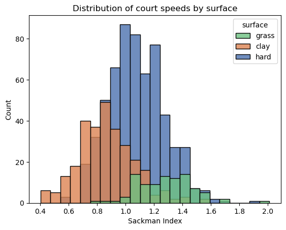
And here is a table of summary statistics for the data since 2006.
| Statistic | value |
|---|---|
| Count | 971 |
| Mean | 1.034 |
| Standard Deviation | .231 |
| minimum | .400 |
| 25th percentile | .872 |
| Median | 1.021 |
| 75th percentile | 1.193 |
| Maximum | 1.945 |
For the most part, these numbers are boring. They tell us grass courts are fast and clay courts are slow, two things we already knew. Yet, the more Sackman indices get right, the closer we should listen to them. The statistic has enough credibility so when it says something counterintuitive, but plausible, we should listen.
And it does have some counterintuitive things to say. For instance, Stuttgart is a clay court tournament, but, according to the Sackman index, it consistently plays quicker than many hardcourt tournaments. Is this plausible? I think so. Notice Stuttgart is played indoors, which quickens the conditions regardless of surface. Players find it easier to hit cleaner (and harder) when the ball is unmolested by the elements. The list of prior champions is also not necessarily what you’d expect of a clay tournament. While Iga Swiatek, who’s strongest on clay, has won the previous two years, Ash Barty, Petra Kvitova, and Angelique Kerber have all won within the last decade. (Kerber, twice). The latter three prefer faster surfaces, so perhaps the Stuttgart conditions are quicker. I think the Sackman indices are suggestive here, but not definitive. At the least, it’s plausible Stuttgart may play surprisingly fast.
The numbers also say something strange about Wimbledon: In 2018 and 2019, it didn’t play fast. In fact, they claim Stuttgart — a clay tournament — played faster. I can only speculate on the cause of a Wimbledon slowdown (the weather?). However, the tournament results for 2018 and 2019 lend some credence to the idea. In 2018, Kerber — who prefers grass — won the title, though there were some surprising outcomes. Dominika Cibulkova — who prefers clay — made a the quarterfinals, and Julia Gorges — who also prefers clay — made the semifinals. In 2019, Simona Halep, “no one’s idea of a grass-court player” according to the New Yorker, won the title, indicating the courts may have played slower.
Long term trends and limitations
The prevailing view is court speeds have slowed over in the last two decades. With Sackman Indices, we can probe this claim. I say “probe” rather than “test” because Sackman indices are not ideal instruments to compare court speeds over time. Remember, the Sackman index is a measure of how many aces are hit in a tournament relative to how many we’d expect given who’s in the draw. This means it’s directly measuring whether WTA players are serving better, or worse, than average. We then use the information on serving to make inferences about court conditions, but there’s no necessary connection between the two. For instance, if WTA players just started serving better without any corresponding change in court conditions, the Sackman index would go up. If we then paraded around saying “courts are getting faster because the Sackman index said so,” we’d be wrong.
It’s also tricky to compare Sackman indices across time. A Sackman index for, say, the 2011 Australian Open is calculated by measuring how many extra (or fewer) aces were hit, relative to player ace statistics prior to that Australian Open. A Sackman index for the 2013 French Open was calculated relative to player ace statistics prior to that French Open, which includes information about aces in 2011, 2012, and 2013. In other words, the two statistics may have wildly different baselines which makes them difficult to compare.
An example illustrates the point. Imagine a simplified WTA tour with one player and two tournaments. The player is Belinda Bencic. The tournaments are Adelaide 1 and Adelaide 2. Both are played at the same location on the same courts in the same conditions. Suppose Bencic’s career ace-per-match statistic is 5. She plays Adelaide 1, and the courts are fast, so she hits 10 aces. Wow! Great for Belinda. Since we observed double the number of aces as expected (10, as opposed to the expected 5), the Sackman index for Adelaide 1 is 2. Now, suppose Bencic’s performance increases her ace-per-match stat to 7.5. She then plays Adelaide 2, and again, hits 10 aces. However, because her ace-per-match statistic has increased to 7.5, the Sackman index for Adelaide 2 is only 10/7.5 = 1.3. For two tournaments with the same courts, player, and aces, their indices differ dramatically.
Hopefully, the example demonstrates how fraught comparing these indices can be. Each Sackman index only makes claims about court speeds relative to what happened before. A Sackman index computed for, perhaps, the 2015 US Open depends on how many aces players hit per match earlier in 2015. An index for 2016 depends on how many aces they hit per match earlier in 2016. 2015 may have been a much different year ace-wise than 2016, so it may be irresponsible to compare the two indices.
At best, I think Sackman indices proxy how fast/slow a tournament plays relative to others in the last 12 months. If the 2015 US Open clocked a 1.1 and the 2016 US Open measured 1.2, it’s difficult to say which one actually played faster. However, I’ll venture the 2016 edition was quicker, relative to the other tournaments in the season, than the 2015 one.
With these caveats in mind, let’s look at Grand Slam conditions over time.
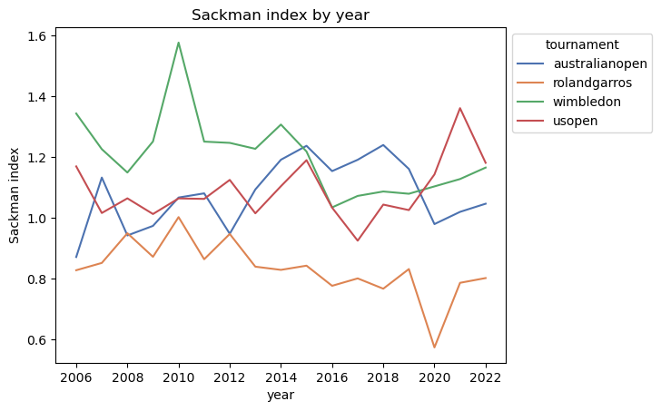
I see a convergence near 2015. Prior, the data match our intuitions. Roland Garros is the slowest and Wimbledon is the fastest, with the hard court slams in the middle. There’s a slow increase in relative speed for the hard court slams, and then the Australian Open, Wimbledon, and the US Open nearly touch. The latter two decline in tandem, leaving the Aussie as the fastest slam of the bunch until the US Open takes the mantle in 2020.
Obviously, we have questions. Why did Wimbledon decline in (relative) speed near 2015? Why did the Aussie and US Open reach local maxima around the same point? Why did the Aussie retain its relative position, but the US Open declined with Wimbledon? Why did the US Open spike in relative speed in 2021? These trends seem unrelated to the speeds of other tournaments. Plotting Sackman indices for WTA 1000 events over time is not illuminating.
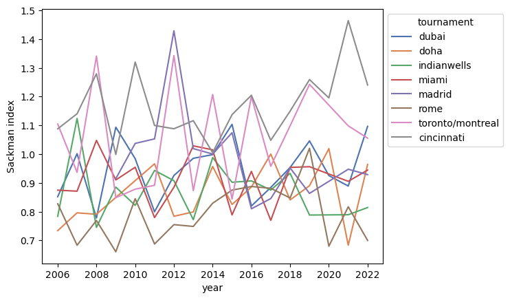
(Remember: the Canada Open switches between Toronto and Montreal every year. The fact Sackman indices record major changes in court conditions corresponding to the change in venue is a point in its favor)
Plotting tour average Sackman indices by surface is also boring:
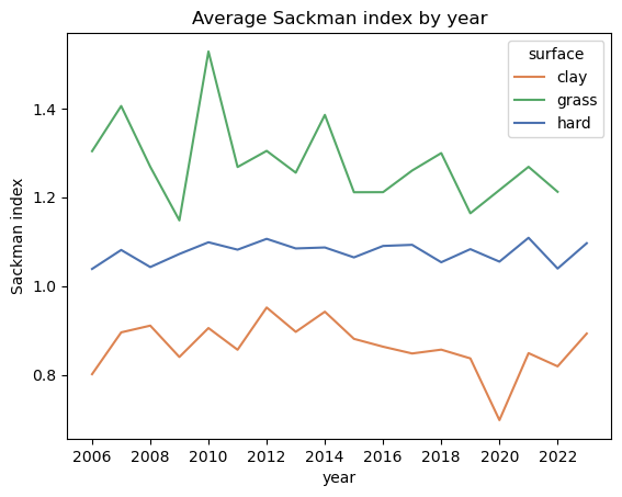
If we squint hard enough, we can imagine/see a small downward trend in the grass Sackman indices. If you’re prone to engage in such squinting, please remember the trend is slight and our sample size of grass matches every year is small. Personally, I would not draw any conclusions from this graph.
Parting words
I like Sackman indices. They match our intuitions about court conditions well, while also suggesting where our we may err. They’re also conceptually simple and rely on public data. The only tricky part is interpreting the numbers. It’s tempting to see Sackman indices as a magical measure of absolute court speed, where an index calculated in 2007 is directly comparable to one calculated in 2017. I argued earlier this view is wrong. First, Sackman indices aren’t necessarily tied to court conditions. They rely on serving performance, which could fluctuate independently of what’s happening on court. Second, they’re calculated relative to contemporaneous conditions on tour, which means numbers from 2007 and 2017 are incomparable. At best, if Doha scores .87 in 2007 and Cincinnati scores 1.24 in 2017 we can say Doha played slow for its year and Cincinnati fast for its own.
If you have any questions or comments, please write me. I’m entering a career in statistics/data analysis and want to improve the best I can. I’m reachable at rileywilson1@protonmail.com.
-
Sackman’s exact methodology is described here. He accounts for the quality of returners in a tournament and surface in his statistics. In the interest of simplicity, I do not. ↩︎
-
The data actually allow me to calculate Sackman indices for tournaments since 2003. However, there are so few observations from the years 2003-2005 that I’m uncomfortable using them. Below is a graph of tournaments I can compute Sackman indices for, per year, which visualizes the disparity.
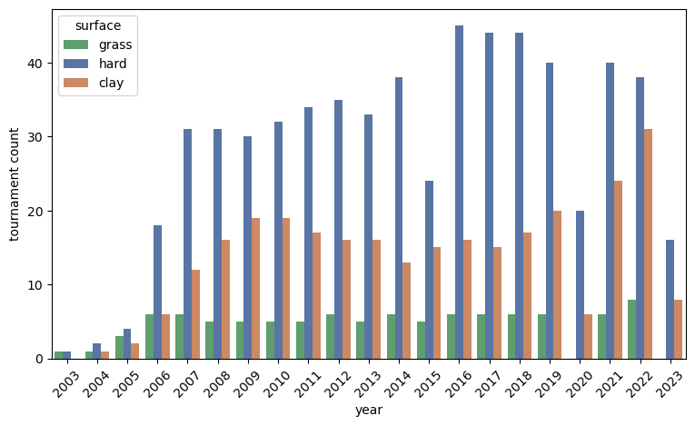 ↩︎
↩︎