The code used for the simulations can be found here.
I.
Imagine there’s a tennis match in Kyrgyzstan between two players you’ve never heard of. You don’t know their rankings, match histories, or even what they look like, but you’re tasked with predicting who will win. The only piece of information at your disposal is player1 has a p chance of winning any given point against player2. In other words, if player1 and player2 played 100 points, on average player1 would win p*100 of these points.
Given only the information above, who do you think will win? How confident should you be they will win?
I’m sure there’s a mathematical pen-and-paper way to solve this problem but we’re going to rely on computer simulations. We can understand how likely it is player1 will win by simulating some large number of matches between both players while factoring in player1’s chance of winning any given point. Our confidence in player1 is represented by the proportion of matches she wins out of the large number simulated.
Here’s an example. Suppose we know player1 has a .51 chance of winning any given point against player2. At 15-0, she has a .51 chance of winning the next point and going up 30-0. At 0-40, she has a .51 chance of getting to 15-40, but a .49 chance of losing the point and the game. To determine our confidence player1 will win an entire match, we might simulate 1000 such matches between player1 and player2 and count how many player1 won. For instance, she might win 586 of the 1000 matches. As a result, if all we know is player1 has a .51 chance of winning any given point, we might say we are 586/1000 = 58.6% confident she will win the match.
The model we consider does this for a specific type of tennis match. All simulated matches are best-of-3 sets with a 7-point tiebreaker played at 6 games all. What’s more, the deuce is “played out,” meaning players must win by two points in order to win a game. I chose this format because it’s the most common type played on the ATP and WTA tours.
We run the simulation and graph the results. 3000 matches were simulated for 50 probabilities on the interval [.4, .6].
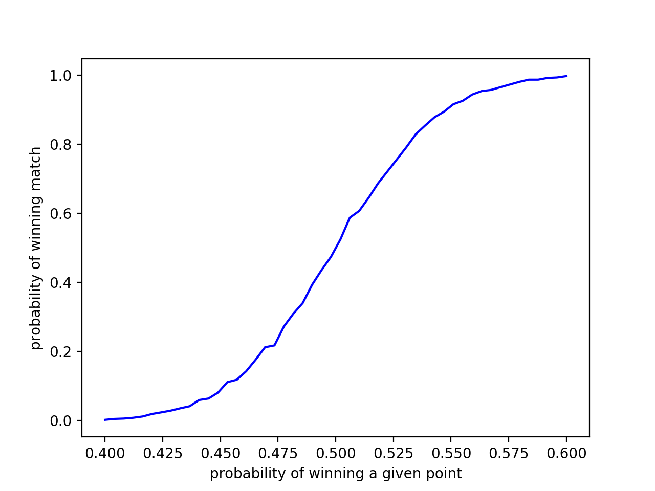
Figure 1 plots the probability player1 has of winning any given point against the probability she wins the match. For instance, if she has a .4 chance of winning a point, it’s very unlikely (~0% chance) she will win the match. Likewise, if she has a .60 chance of winning a given point, her probability of victory is ~100%.
As expected, if player1 has a .5 chance of winning a point, she has a 50% chance of winning the match. Based on this, we might expect a .525 chance of winning a point to yield a 52.5% chance of victory. Yet, our intuition fails to grasp the benefits of a slight edge. Just increasing the probability of winning a point from .5 to .525 causes the probability of winning the match to increase from 50% to 75%! A .025 increase in win probability at the point level leads to a 25% increase at the match level. To put this in perspective, we might say the difference between a player that wins 50% of her matches and one that wins 75% of them is the latter wins 2.5 more points out of 100 than the former. To make it even more concrete, we can surmise the difference between Pete Sampras (64 career singles titles) and Carl-Uwe Steeb (3 career singles titles) is only 2.5 points per 100!
Fully explaining Pete Sampras’ dominance and Carl-Uwe Steeb’s adequacy is far beyond the scope of our model, though. At best, we can say a player with a .525 point win rate would have a match record like Sampras’. However, this does not imply Sampras actually won 52.5% of the points he played, or a player who does win that proportion will be a 14-time grand-slam champion. We are only noting similarities between the statistics of idealized players considered in the model and actual ones. Resemblance only suggests both players could have other common properties.
Still, the results are striking. Player1 only needs a .55 probability of winning a given point to win ~95% of the matches she plays. Approaching .6 almost guarantees she’ll win every time. Even a .51 probability of winning a point increases the odds of winning to ~.6.
Any tennis player will tell you the margins are slim, but now you’ve seen it computationally demonstrated. Common tennis platitudes like “every point counts” and “make them work for each point” take on additional significance. The practical implication is to focus more on individual points as opposed to games or sets when playing a match. Any competitive tennis player should already do this, but now they have an additional, semi-scientific reason to do so.
Back to Kyrgyzstan. We understand player1 has a p chance of winning a given point. If p > .5, we should be confident she will win. If p > .525, we should be really confident she will win. The same holds on the other side of .5. If p < .475, we should root for an upset. If p < .45, there’s pretty much no hope.
There’s another match happening in Zanzibar. We still know player1 has p chance of winning any given point, but now we know something else: she chokes. Whenever she has game, set, or match point, her probability of winning said point drops from p to pc. As an example, imagine her p = .55 and pc = .35. Suppose she’s also up 40-15 in a game against player2. Although her probability of winning a given point is .55, because it’s a game point, there’s only a .35 chance she wins the next point to secure the game. If she was up 6-4 in a tiebreaker, the same decrease in probability occurs. There’s only a .35 chance she wins the tiebreaker 7-4.
A similar problem presents itself. Given player1’s p and pc, will she win the match? How confident should we be in our prediction?
We run the same model in the previous section with some minor modifications. Whenever player1 is poised to win a game, set, or match, her probability of winning the next point plummets to some pc. As in the previous section, we vary p within [.4, .6] and observe player1’s probability of winning the match. What’s different now is each curve is associated with a constant pc.
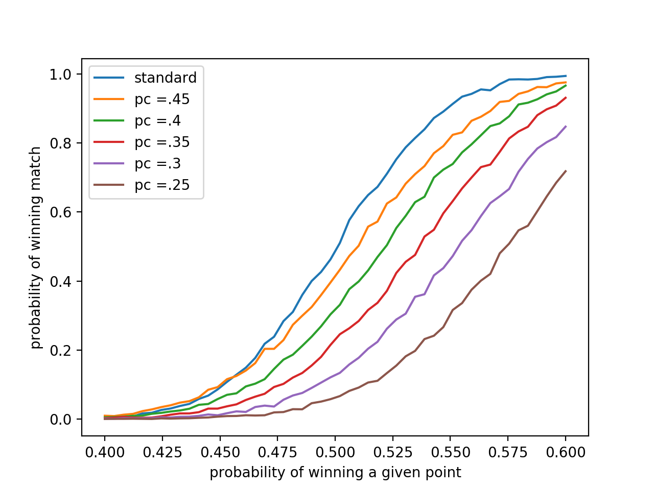
The blue “standard” curve represents how player1 would perform sans choking. It is the same curve depicted in Figure 1 where her probability of winning a given point is p regardless of the score. The others record what a player’s match record at a certain p would be like given her pc. If player1’s pc = .45 for instance, her performance suffers heavily. At p = .5, she has only ~40% chance of victory compared to the 50% chance observed with an identical p in the absence of choking.
Past p = .5, a .05 decrease in pc roughly corresponds to a 10% reduction in the chance of winning a match. If player1’s p = .525, and pc = .45, her chances of winning would be 62%. However, if her mental game falters and pc drops to .4, her chance of victory decreases to 53%.
Clearly, any level of choking impedes performance. If we know player’s pc is low, we should expect a rather large p to compensate. Player1’s coach might suggest addressing the root factors of unclutchness. A sports psychologist or deep reflection might increase pc, or eliminate choking altogether.
There’s a third tournament in Andorra and we’ve learned more about player1. She no longer chokes at this junction in her career, but her play has become streaky. Given she won the previous point in a match, there’s a probability ps she will win the next point as well. If ps = .8, for example, there’s an 80% chance she will win the next point after winning the previous one. However, streakiness goes both ways. Given she lost the previous point, there’s an 80% chance she will lose the next one as well. The first point of every game (and tiebreak) is a fresh start, though. The chance she wins that point is p. From then on, ps reigns.
To get a sense of our credence in player1’s performance, we run another simulation.
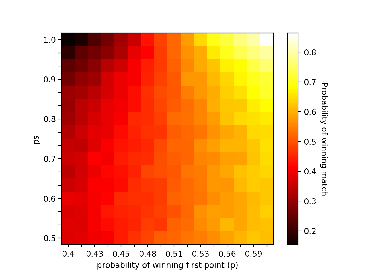
This is a heatmap. The color of the block occupying the (probability of winning first point, ps) coordinate corresponds to the probability of winning the match. Light colors indicate high probabilities while darker colors represent low ones. As an example, if player1 has a .42 probability of winning the first point of any given game or tiebreaker and her ps = .9, her probability of winning the match is around .3. Here, we note heatmaps favor concise representation over numerical precision. The bar on the right gives us only a general idea of what probabilities are associated with which colors.
Still, patterns are clear. Variation in ps only has noticeable consequences at the extremes. If p is low, then a high streakiness almost guarantees losing the match. Observe how the probability of victory is only ~20% when p = .4 and ps > .9. However, for any value of ps < .9, the probability of winning the match hovers around 40% if p remains fixed. Similar results occur for higher p’s. Only when ps is large do we see its influence on chance of victory. At values of p close to .5, ps has no apparent effect. The probability of winning the match stays roughly constant as ps varies.
It might look like high ps, or streakiness, is an advantage when p is sufficiently greater than .5. This is true, but the gain is comparatively small. Recall the Kyrgyzstan model where player1’s probability of winning the next point was constant throughout the match. If p = .525, player1 had 75% chance of victory. Here, for all levels of ps, p = .525’s probability of victory hovers around 60%. Player1 is much better off winning 52.5% of points in general as opposed to embracing streakiness.
We should note streakiness as we’ve defined it “smooths” performance at low values of ps. If ps = .5, this means players have a 50% chance of winning any given point after the first. In other words, we’re saying the players are just about even after the initial point. If p = .4 in the Kyrgyzstan model, a player has almost no chance of winning. In this model, p = .4 gives an ~40% chance. What it captures at these kinds of values is the dynamics of one player frequently winning the first point, and then both players having an equiprobable chance of winning the following ones.
We take these results to Andorra. Streakiness only concerns us at the extremes. If player1 has an exceptional chance of winning the first point and is very streaky, we’re confident. If she’s dismal on first points but just as streaky, we lose faith.
II.
I’m excited about these models for two reasons. First, they suggest other interesting questions to tackle. How do the probabilities change in 5-set matches? What about no-ad? What if a player is brilliant on break points? What happens if we incorporate a serving advantage? Can we combine several of these models? The list goes on.
The second reason is epistemological. Can models of this type provide ever provide an explanation of real-world phenomenon? I talked about the Kyrgyzstan model being insufficient to explain Pete Sampras’ dominance, yet, there are distinct reasons why people may think this is so. We could say to explain Pete Sampras’ skill, we must address specific aspects of his game. It’s necessary to observe his deft touch at net, booming serve, and flat forehand. Pete Sampras is good, the reasoning goes, because he was able to hit aces and put away volleys. Any explanation of Sampras’ skill has to begin with these factors. Under this perspective, the Kyrgyzstan model fails to give an explanation because it is too abstract. Only tracking the probability of winning any given point obscures the unique advantages Sampras had that contributed to such a high probability. Proponents of this critique believe, in principle, no idealized model can explain why a given tennis player was so successful. Such models are incapable of capturing the unique, individual aspects of a player that contributed to his or her dominance.
A second critique finds no fault with idealized models in general — just the Kyrgyzstan one. It claims idealized models can give explanations of real-world phenomena, but this one in particular is too weak to do so. A model that actually provides an explanation would take parameters like probability of winning break points, probability of saving break points, probability of winning a point on second serves, probability of winning games/sets when down or up, etc… It would be much more detailed, but it still wouldn’t directly address the unique aspects of Sampras’ tennis the prior camp requires. Explanations from the model would sound like “Sampras was great because he had a high win percentage on second-serve points,” or “Sampras was a champion because he had a high probability of saving break points.”
This camp believes idealized models can supply these explanations and they’re sufficient for deep knowledge. To understand Sampras, we only need to understand his propensity to win or lose in general scenarios. We only care about his serve or volleys or movement insofar as they contribute to a high break-point save rate, for instance. The statistical measures provide the base of our understanding; everything else is secondary.
We might be partial to a certain type of explanation. Players and coaches will tend to explain matches in terms of backhands and serves where statisticians will invoke probabilities and win rates. Our intuitions are often with the players. We find it hard to believe understanding Djokovic is possible without seeing a sliding open-stance backhand winner, or a kick-serve that bounces over your head in the case of John Isner.
Are our intuitions correct? Are the modelers correct? Which level of explanation gives us the best understanding of a tennis player? Is one of these levels subordinate to the other?